Geophone Response

The geophone consists in a mass dangling from a spring attached to a frame coupled to the Earth. Around the mass there is a magnet. When the Earth moves suddenly, the mass tends to remain stationary and will lag behind the motion of the Earth. The resultant voltage is proportional to the velocity of this motion. The oscillation will gradually die due to losses in the magnetic circuit : if the coil is loaded or shorted, the current will cause a force that will oppose the motion : damping.

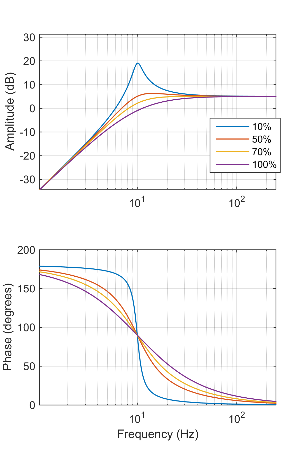Geophone Responses for several damping coefficients.

The geophone is a single degree of freedom harmonic oscillator with a mass, a dashpot and a spring : \[F=m\ddot{x} + c\dot{x} + kx\]

Where \(F\) is the Force (\(N\)), \(m\) the mass (\(kg\)), \(x\) the displacement \((m)\), \(c\) the damping (\(kg.s^{-1}\)) and \(k\) the spring constant (\(kg.s^{-2}\)).

The Laplace transform of this equation is : \[F(s)=ms^2z(s)^2 + csz(s) + kz(s)\]

Solving for the transform function : \[\frac{z(s)}{F(s)}=\frac{1}{ms^2+cs+k}=\frac{1/m}{s^2+s.c/m+k/m}\]

Substituting the following variables : the resonant angular frequency \(\omega^2_n = \frac{k}{m}\), the critical damping \(c_{cr}=2\sqrt{km}\) and \(\zeta\) a percentage of the critical damping, the equation is re-arranged : \[\frac{z(s)}{F(s)}=\frac{1/m}{s^2+s.2\zeta\omega_n+\omega_n^2}\]

The frequency response is computed by substituting \(s\) by \(i\omega\) \[\frac{z(iw)}{F(iw)}=\frac{1/m}{(i\omega)^2+i.2\zeta\omega\omega_n+\omega_n^2}=\frac{1/m}{-\omega^2+i\omega.2\zeta\omega_n+\omega_n^2}\]

NB: When the damping percentage \(\zeta\) equals \(\frac{\sqrt{2}}{2}=0.714\), the denominator corresponds to a 2nd order Butterworth filter polynomial.

The impulse is the integral of the force (Impulse and Momentum theorem), and the voltage recorded by the seismometer is proportional to the velocity of the coil in the geophone, so the expression has to be derivated twice to get a seismic impulse response: \[IMP(iw)=(iw)^2.\frac{z(iw)}{F(iw)} = \frac{1/m}{1-i2\zeta (\omega_n/\omega) - (\omega_n/\omega)^2}\]

Matlab example

Here is a quick example to compute the time-domain and frequency-domain impulse response of a geophone given its damping and resonant frequency.

	% This computes the normalized Impulse response for a Geophone, in velocity
	% domain
	Damp = sqrt(2)/2; % percentage of critical damping
	f0 = 10; % resonant frequency (Hz)
	L = 4; % record length (seconds)
	Si = 0.002; % sampling interval (seconds)
	Ns = L/Si; % number of samples
	Nf =  ceil( Ns/2) +1 - mod(Ns,2); % number of positive frequencies after FFT
	% sample the frequency scale 
	fscale = [0:floor(Ns/2)]/Ns/Si; 
	fscale = [fscale -fscale(end-1+mod(Ns,2) : -1 : 2)]';
	% compute the IRs
	IMP = 1./( 1 - 1i.*2.*Damp.*(f0./fscale) - (f0./fscale).^2); % frequency-domain impulse response
	IMP_t = real(ifft(IMP)); % time-domain impulse response
	figure,plot(IMP_t(1:.5/Si)) % plot first half-second in time-domain

References

Andrew Pap. Criteria for the selection of geophone parameters, hookups, phone spacing, and lowCut instrument Filters, pages 472–475. 2005. doi : 10.1190/1.1894056. URL

G.C. Drijkoningen. Seismic data acquisition. ta3600, 2003. Delft University of Technology.